Conditional formatting
Conditional formatting, as the name implies, is about formatting a cell based on some preset conditions. These conditions could be based on the content within the cell or from some other cells. We can define up to 3 different formats for 3 different conditions in each cell (For Excel 2003 and below. Excel 2007 and above can perform unlimited conditional formatting). For example, you could use conditional formatting to monitor whether salespersons fall short, meet
or exceed their sales targets. Here is an example on how we can set these targets
Setting the conditional formats based on the value (actual sales as a percentage of the sales target) within the cell.
1. Select the cell you wish to set the conditional formatting.
2. Click on Format on the menu, followed by conditional formatting
3. A dialog box will appear as shown:
4. Set the first condition (fall short of sales target) by selecting “less than or equal to” instead of using the default “between” option using the drop down button. The 2 text boxes on the right would be replaced by one single text box. Enter the value “90%” into the text box. This means that the salesman will be considered as falling short of the target if the actual sales achieved by him is less than or equal to 90% of the sales target. Click on the format button and define the format (for fonts, cell border and colors & patterns) you want Excel to show when the condition is met. One suggestion is to format the cell “red”.
5. Next click on the Add button to create a second condition. In this second condition, leave the “between” option as it is, enter the value “90%” and “110%” into the 2 text boxes. Click on the format button (for condition 2) and preset the format for this range. In our example, let’s assume that there will be no change in format if the percentage falls within this range.
6. Click on the Add button, and make the cell turns “green” format if it meet the 3rd condition, i.e. “>110%”.
7. Click on the OK button when you are done.
8. Once the conditional formatting for the cell has been set, we will be able to monitor the salespersons performance using the cell’s color code. If the cell turns red, we will immediately know that the salesperson has achieved less than or equal to 90% of the sales target. If the cell shows a normal format, they are within target. If it turns green, the salesperson has exceeded the sales target.
Setting the cell format based on conditions in another cell
1. Select the cell you wish to set the conditional formatting.
2. Click on Format in the menu, followed by conditional formatting.
3. A dialog box will appear as shown:
4. Click on the drop down box on the left of the dialog box and change the option from “Cell Value is” to “Formula is”. The last 3 dialog boxes would be replaced by one single dialog box.
5. Assuming that the cell you want to set up the conditional formatting is cell A1 (e.g. salesman’s name), and the percentage of actual sales against the sales target is found in cell C1.
6. Enter the formula into the text box as shown:
7. Do the same for the condition on meeting the target and another condition for exceeding the target.
As the value in cell C1 changes, the format in cell A1 will change accordingly.
An example
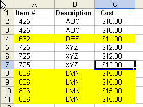
Given below is a list of stock items:
Anytime the Item # changes I want to highlight the row, as in the above example: The first 2 lines would not be highlighted, the third line would be, then lines 4,5,6 would not be highlighted, the last 4 items would be highlighted.
1. Select Cell A2.
2. Go to menu -> Format -> Conditional Format.
3. Change the option from cell value is to “formula is”.
4. In the formula field, enter the following formula without quotes
“=IF(MOD(SUM(IF(FREQUENCY(IF(LEN($A$2:$A2)>0,MATCH($A$2:$A2,
$A$2:$A2,0),””),IF(LEN($A$2:$A2)>0,MATCH($A$2:$A2,$A$2:$A2,0),“”))
“=IF(MOD(SUM(IF(FREQUENCY(IF
(LEN($A$2:$A2)>0,MATCH($A$2:$A2,$A$2:$A2,0),””),
IF(LEN($A$2:$A2)>0,MATCH(
$A$2:$A2,$A$2:$A2,0),
“”))>0,1)),2)=0,0,1)”.
>0,1)),2)=0,0,1)”.
Without fixing the row allows us to copy the format down to the rest of the list)
5. Format the cell based on your preference by clicking on the format button located on the right.
6. Copy the format from A2 to the rest of the table.
7. You will notice that the format you indicated appears when the item # changes.
Application of conditional formatting
Adding UP and DOWN arrows next to numbers
New! Comments
Have your say about what you just read! Leave me a comment in the box below.
Share this page:
Enjoy this page? Please pay it forward. Here’s how…
Would you prefer to share this page with others by linking to it?
- Click on the HTML link code below.
- Copy and paste it, adding a note of your own, into your blog, a Web page, forums, a blog comment, your Facebook account, or anywhere that someone would find this page valuable.
<a href=”http://www.advanced-excel.com/”>Advanced Excel – From a Business Perspective</a><a href=”http://www.advanced-excel.com/”>Advanced Excel – From a Business Perspective</a>

Excel Courses for Business Professionals
Copyright © advanced-excel.com 2007 – 2019. All Rights Reserved. Privacy Policy
Microsoft® and Microsoft Excel® are registered trademarks of Microsoft Corporation.
advanced-excel.com is in no way associated with Microsoft


