Create a dynamic Excel Calendar without macro
We wanted to plan for our excel course schedule originally with a paper calendar but couldn’t find one. It was too early in the current year to find a paper calendar for the folloiwng year. So we decided to create a simple calendar manually using Excel but find it especially tedious to do so. We have to constantly keep track of the starting and ending day of each month. Then we have to manually color the holidays and the school holidays. And if we happen to mark out the dates wrongly, we have to
re-do the holidays all over again. So out of desperation, I started to google for such an excel calendar and found many. Most of them are free. But they were not really impressive because they have to be generated either through Excel macro/vba or a third party program. I feel that it will not go well with most excel users because they would have to understand how to activate the macro or installing another program in their computers. If it is created manually without using any program, it is going to be time-consuming because we need to identify the 1st of every month manually first and then doing manual summation to populate the rest of the days of the month. Furthermore, we have to consciously stop the calendar from going beyond the legitimate 28, 29, 30 or 31 days for the month.
As I continue to search through the list, I stumble on this perpetual calendar from John Walkenbach and was amazed by the way it was created. It is a perpetual excel calendar because it can be used for ANY year. It uses only excel formulas, which means that you do not need to know anything about macro and it can be run using different versions of Microsoft Excel including the latest version of Excel. If you are keen to use the template straight away, then go to this Excel calendar page to request for it. If you wish to learn some Excel formulas and how this calendar is created, read on. We are going to show you how it is done step by step.
1. Download the excel calendar template by click on this excel calendar link.
2. Enter the year 2009 into cell C3 in the template.
3. In cell C5, enter the formula “=DATE(C3,1,1)”. The formula will create the date for the first day and the first month for the year in Cell C3, i.e. 1 Jan 2009.
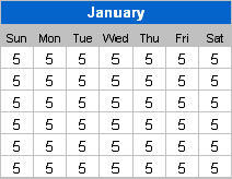
4. Select the range C7 to I12. There should be 6 rows and 7 columns. 6 rows because a month may span across 6 weeks. 7 columns because there are 7 days in a week.
5. Set the formula in the range C7:I12 to present the first day of the month. You can use the date formula for this. In our case, we can enter the formula as “=$C$5”. C5 refers to 1 Jan 2009. Use the key CTRL + ENTER to enter the formula into the whole range, all at one go.
6. Identify the day of the week for the 1st day of the month. Use the weekday formula to identify the day of the week for the first of the month. Change the formula in the range C7:I12 to =WEEKDAY($C$5)The weekday formula presents the week with Sunday as the 1st day of the week and Saturday as the 7th or the last day of the week.
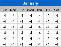
7. Minus one from the weekday formula, we will get Monday as 1 and sun as zero. 1 Jan 2009 is a Thursday which coincides with the number 4.
The Sunday before 1 Jan 09 is actually 28 Dec 08 which is 4 days before 1 Jan 09. So, when we insert a minus sign before the formula created in the previous step, it will return -4. You may have to change the cell format to General to see the number (do this if ### appears in all the cells). And the results for using the formula =-(WEEKDAY($C$5)-1) are
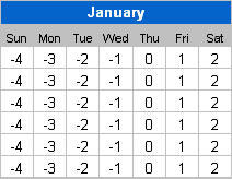
8. The Sun on the top right hand corner is 4 days earlier than 1 Jan 2009. Monday should be 3 days earlier and Tue 2 days earlier. Therefore, in this step, we need to make the number increase over the week starting with -4. To do this, we need to enter the formula as an array formula, which will compute the result based on the cells in the whole range. An array formula comes with curly brackets (special case here) which can only be created by pressing the 3 keyboard keys (Ctrl + Shift + Enter) together. Make sure the range C7:I12 is selected when the 3 keys are pressed together.
Add the formula +{0,1,2,3,4,5,6} at the end of the formula. Press CTRL + SHIFT + ENTER again (make sure the range C7:I12 is selected). In this revised array formula, the curly brackets indicates that the number to be added to each cell is from 0 to 6, depending on the position of cell in the range (horizontally). The first cell on the left should add the value 0, second cell 1, etc. The picture below shows you the result you should be getting in this step.
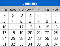
9. In the second row/week of the month, the value should continue from the last value in the previous row. Since there are 7 days in a week, we know that the first value in the second row should be 7 days more than the cell above it. We can add another array using semi-colon (;) to indicate that we want the number to increase as the row increases. It should be presented within curly brackets and multiply by 7 – {0;1;2;3;4;5;6}*7. We should not add any number to the first row. Then the second row should add 7 to the number and add 14 to the third row and so on.
The formula is
=$C$5-(WEEKDAY($C$5)-1)+{0;1;2;3;4;5}*7+{1,2,3,4,5,6,7}-1
10. To convert the results above into real dates, we can add the date 1 Jan 2009 into the box. In this case, the first number will become 28 Dec 08, 29 Dec 08, etc. And 32 will become 1 Feb 2009. We can insert the $C$5 immediately after the equal sign. And to display the day of the month only, we can format the cell with using the custom format “d”.
11. To omit the Dec 08 dates and Feb 09 dates, we can compare the month of the date with the month used in the first day of the month, etc. If they are different, it means that the date shown in the active cell belongs either to the previous month or the following month. We can put a blank(denoted by open and close inverted comma) into the cell (all the cells). If the month of 2 dates are the same, continue to perform the calculation given in the previous step. We will end up with the following formula:
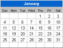
=IF(MONTH($C$5-(WEEKDAY($C$5)-1)+{0,1,2,3,4,5,6}+{0;1;2;3;4;5;6}*7)<>MONTH($C$5),””,$C$5-(WEEKDAY($C$5)-1)+{0,1,2,3,4,5,6}+{0;1;2;3;4;5;6}*7) This completes the creation of the excel calendar template for the month of January:
12. Remove the $ in $C$5 by using Find ($C$5) and replace (C5). Copy the formula to the other 11 months. Change the date in the month header to correspond to the relevant month.
13. Using the formula version of conditional formatting, enter the VLOOKUP and ISNA formulas to find whether there is a match in the list of public holidays. If there is, change the color of the cell to red. In the excel calendar template, a more complex vlookup formula is used to check if the public holiday falls on a Sunday. If it is a Sunday, it will color Monday red instead of Sunday.
14. Using the same conditional formula concept, enter the important dates and set the color of the cell if there is a match in the date. The second condition will be validated only if the first conditional formatting condition fails. This means that if your important date falls on a public holiday, it will be highlighted red instead of the color you specify here.
You can request for a FREE copy of the excel calendar if you decided to wish to use it right away!