


Auto-Highlight Records Through Conditional formatting for Excel 2007 and Excel 2010
Auto-highlight a row can be easily achieved if you know conditional formatting in Excel. As the name implies, it is about formatting a cell based on some preset conditions. These conditions could be based on the content within the cell or from some other cells. In Excel 2007, there is no limit on the number of conditions you can define for the cell. Here is an example on how the conditional format can auot-highlight dates.
In the picture below, we wish to highlight the rows RED when the date displayed in column C that is less than 30 dates from today and highight YELLOW when it is more than 30 days but less than 60 days from today.

Using conditional formats to auto-highlight the rows.
1. Select the range A2:D5 you wish to set the conditional format.
2. In the Home Tab/Ribbon, click on Conditional Formatting.
3. In the dropdown menu, select Manage rules.
4. In the pop-up window, click on the button “New Rule”.
5. In the next pop-up window, choose the rule Type “Use a formula to determine which cells to format. In the box below, we enter the first rule for Red colour. Type in without quotes
=($C3-TODAY())<30
Take note of the dollar sign. There isn’t one before the number 3. This is to make the conditional format function look for the relative dates in the subsequent rows. The TODAY() formula will all use today date for the calculation. Then click on the Format button to set the format to fill the cell with RED when the condition is met. Click on the OK button twice to go back to the window titled “Condtional Formatting Rules Manager”
6. Click on the “New Rule” button again.
7. In the next pop-up window, choose the rule Type “Use a formula to determine which cells to format. In the box below, we enter the 2nd rule for Yellow colour. Type in without quotes
=AND(($C3-TODAY())>=30,($C3-TODAY())<60)
The AND formula is to make sure than both conditions (separated by comma) must be met before the conditional format will highlight the cell yellow. Then click on the Format button to set the format to fill the cell with YELLOW when the condition is met. Click on the OK button twice to go back to the window titled “Condtional Formatting Rules Manager”
8. In the “Condtional Formatting Rules Manager” window, check on the box below the decription STOP if TRUE. This is to stop conditional formatting from checking the condition once the condition is met. Click Apply and Close.
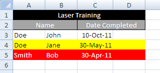
Now, row 4 is auto-highlighted with YELLOW because the DATE COMPLETED is more than 30 days but less than 60 days from TODAY (calculation done on 14 Apr 2011).
Row 5 is highlight RED because the DATE COMPLETED is less than 30 days from TODAY.
Because we enter the formula TODAY() as part of the condition, the check will refresh on a daily basis and auto-highlight the cells using today’s date as a reference.
Introduction to auto-highlight / conditional formatting

New! Comments
Have your say about what you just read! Leave me a comment in the box below.
Share this page:
Enjoy this page? Please pay it forward. Here’s how…
Would you prefer to share this page with others by linking to it?
- Click on the HTML link code below.
- Copy and paste it, adding a note of your own, into your blog, a Web page, forums, a blog comment, your Facebook account, or anywhere that someone would find this page valuable.
<a href=”http://www.advanced-excel.com/”>Advanced Excel – From a Business Perspective</a><a href=”http://www.advanced-excel.com/”>Advanced Excel – From a Business Perspective</a>

Excel Courses for Business Professionals
Copyright © advanced-excel.com 2007 – 2019. All Rights Reserved. Privacy Policy
Microsoft® and Microsoft Excel® are registered trademarks of Microsoft Corporation.
advanced-excel.com is in no way associated with Microsoft