Offset Function
The OFFSET function is used to return the address of a cell or a range of cell through the use of a reference cell. If we know the cell or range beforehand, we are unlikely to use it at all. It is very useful in our spreadsheets when we do not know the cell or the range of cell in advance, especially in situations where you allow the spreadsheet to interact with the users such as preparing a business dashboard that reports on the performance of a product from a list.
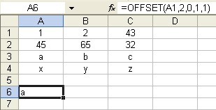
In the above diagram, cell A6 contains the character “a”. If you look at the formula bar, you will notice that the character “a” was not typed into the cell. Instead, it was a result returned by the offset function. We have basically instructed excel to return the value that is found in cell A3. How was this done?
1. First, we identify a cell as a starting point. This is our base cell. In the formula above, the base cell is A1 in “=OFFSET(A1,2,0,1,1)”.
2. We have indicated in the offset formula that we want the result that is 2 rows below the base cell A1 “=OFFSET(A1,2,0,1,1)”.
3. Next, we also tell the offset formula that the result should be 0 column from the base cell. By now, the offset formula would have identified that we are looking at the cell A3, which is 2 rows below A1 and zero column to the right of A1.
4. Finally, we told excel that size of the range we want is 1 row tall and 1 column high, i.e. a single cell “=OFFSET(A1,2,0,1,1)”.
5. As a result of this instruction, the character “a” was displayed in cell A6.
This result is the same as entering without quotes “=A3” into cell A6.
Note:
a) If you want the offset function to move above the base cell, then enter it as a negative number. In the above example, the offset will return an error because it is unable to find anything above the cell A1 (outside the boundary of the excel worksheet). However, if you have entered the base cell as B3, then you could instruct the offset formula to move 1 row above the base cell. The offset function will return the value “65” as its result. The formula to do this is “=OFFSET(B3,-1,0,1,1)”
b) The smallest size of the result “=OFFSET(A1,2,0,1,1)” is 1 row tall and 1 column wide. In this example, only 1 row and 1 column are used. The size of the range can be increased but the result will show #VALUE! in the spreadsheet. This is because the cell cannot accept a range reference such as this: =C1:C2. To understand this better, you can use it together with another formula such as SUM.
Using OFFSET function within a SUM function
When we increase either the row height or column width in the offset function “=OFFSET(A1,2,0,1,1)” to more than 1, the reference is converted to a range. In this section, we will explain how we make use of the offset function to find out sum of the range C1:C2
1. Set up the offset function such that it is referenced to the cell C1. The formula will start with the base cell A1 “=OFFSET(A1,0,2,1,1)”. To identify C1 as the starting poin (top left hand corner of a range), enter the number 0 to instruct the offset function to stay in the same row 1 “=OFFSET(A1,0,2,1,1)”. Enter the number 2 to indicated that we want to move 2 columns to the right of the base cell A1 “=OFFSET(A1,0,2,1,1)” (Column A is numbered 0). That is Column C. Keep the last two numbers as 1 to indicate that we want the offset function to point to one single cell C1 “=OFFSET(A1,0,2,1,1)”. The result will show the value in cell C1, i.e. the number 43.
2. Enclose the offset function with a sum function “=sum(OFFSET(A1,0,2,1,1))”. The result continues to show 43.
3. As our plan is to sum the range C1:C2, we need to increase the row height to 2 “=sum(OFFSET(A1,0,2,2,1))”. The number now changes to 75. It has included the number 32 in cell C2. The number 75 is the result of summing cell C1 (43) and C2 (32). We have included a diagram below to help you understand better.
Other than using it together with the SUM formula, you can also use the OFFSET function to determine a range automatically.


