Inventory Management System
You can create a simple inventory management system to keep track of your stocks. In this page, we will first share with you how to capture the records of stock movements in and out of a warehouse/retail shop/distribution center in an Excel worksheet. Then we will show you to create a simple report that identifies the stock level of individual stocks at the end of each period. The function we are going to use in here is an advanced application of pivot table.
First create a list with the relevant details. The list should not contained too much details until the person(s) is/are not willing to use it. At the same time, you should bear in mind that the list should contain enough details for your analysis.
In our example, we will only capture the following details:
1. Product Group,
2. Product Name,
3. Pirce,
4. Date,
5. Quantity In,
6. Quantity Out,
7. Location
In this list, the store or warehouse manager must make sure that the above details are keyed in for goods that they received and good sent out or sold. Below are an example of goods coming in (line 1) and going out (line 2).
![]()
At the end of 2 months, your worksheet would have contained a number of records detailing the movement of stocks in and out of the store or warehouse. With the records, you could then create a pivot table showing the quantity of goods in and out of the warehouse. Here is how:
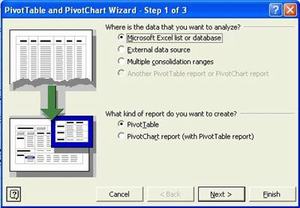
1. Select Data – PivotTable and PivotChart Report.
2. Select the option Microsoft Excel list or database and Pivot Table
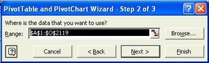
3. Enter the range of the database or list
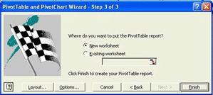
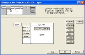
4. When you come to the wizard step 3 of 3, click on Layout button.
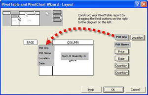
Drag and drop* the fields into the respective places as shown below and click ok.
5. Select the option to put the pivot Table on a new sheet and click Finish You should have a report that looks like this:
Showing the stock movement in the inventory management system using Pivot Table
In our example, we can calculate the net change between the “Quantity In” and “Quantity Out” by using the formula function in Pivot Table. You can only do this using the Pivot Table Toolbar.
1. Select a cell within the pivot table.
2. Click on the right mouse button.
3. Select “Show Pivot Table Toolbar” (if the description is “Hide Pivot Table Toolbar”, it means that the toolbar is already displayed in Excel)
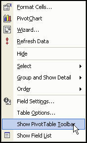
4. The pivot table toolbar should become visible.
![]()
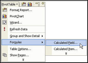
5. Select a cell within the pivot table, click on the label “Pivot Table” in the toolbar and a menu will drop down from the description.
6. From the dropdown menu, select formulas – Calculated field
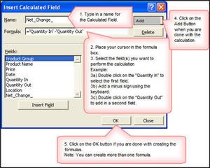
7. In the calculated field dialog box, add in a name for the field.
8. Select the field(s) you want to use to perform the calculation.
9. Click on Add when you have filled in the formula.
10. Click OK to exit the dialog box.
Changing the original Pivot Table Layout
1. Move you mouse over the pivot table and click on the mouse button.
2. Select Wizard.
3. Click on the layout button.
4. Remove the field “Sum of Quantity In”.
5. Click OK and in Step 3 of the pivot table wizard, click Finish.
Summarise the stock movement by Month for the inventory management system
1. Move your mouse over the cell that displays the date header/field and click on the right mouse button.
2. In the pop-up menu, select “Group and Show Detail” – Group
3. Excel will automatically select the full range of the dates you wish to group.
4. Select the groupings (month, quarter, year) you need. You can select more than 1.
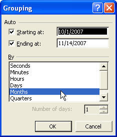
5. Click OK.
6. The details are now summarised by Month.
7. Move your Date field to the column area
8. Click and hold on to the date field.
9. Move your mouse over the cell displaying the total.
10. You will see a box outline covering the “total” cell as shown.
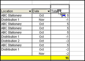
11. Your stock movement is now presented across the columns by month.
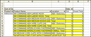
The inventory management system can now present the individual stock level by month
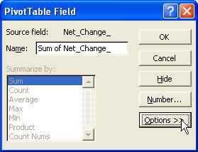
1. Double click on the data field located at the top left hand corner of the pivot table.
2. Click on the Options Button found in the PivotTable Field dialog box.
3. In the “show data as:” box, select “running total in”.
4. In the base field, select date.

5. Click OK.
6. The pivot table will now show the stock level by product for each month.