Create 2 y-axis Excel Chart

Presenting Numbers and Percentages on the same chart

Step One:

Click here to obtain a sample of the excel chart data. Select the data range (B2:D7) for the charts.

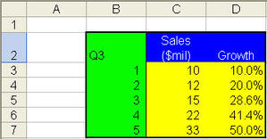
Including the header will ensure that the chart wizard automatically create a link to the headers. This means that you do not have to manually type in the series names into the chart. You can also change the header(s) description easily by change the description on the spreadsheet.

Step Two:

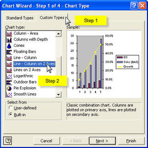
Click on the chart icon. This will activate the chart wizard and go to Step 1 of 4 of the chart wizard. Select the tab called “Custom Types”. Scroll down the list on the left and select the chart type “Line – Column on 2 axes”.

Step Three

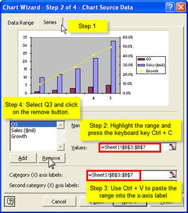
Click on next to go to Step 2 of 4. Use Ctrl + C to copy the range and Ctrl + V to paste the copied range to the x-axis. The x-axis range will be available to all the series. Delete the series Q3 because it is meant to be the range for the x-axis.

Step Four

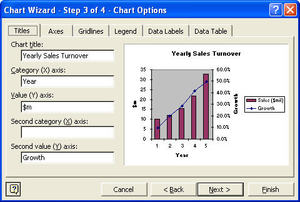
Click on next and fill in the details such as Title, x-axis label, y-axis labels and etc.

Step Five

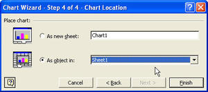
Select to present the chart in the worksheet as an object (preferred).

Note that this chart is static, which means that it does not change until you change the numbers in the table. If you are looking for a chart that will automatically update with the latest figure, you can consider pivot chart. To learn how to make use of Pivot Chart, attend our coming Excel course “Sales Performance Analytics with Excel” and we’ll show you how to do this and many other good stuff you can do in Excel.