How to create a Pivot Table for your survey results
When you receive a set of records, it is very tempting to create a Pivot Table straight away. And you will end up with a Pivot Table report that is not flexible at all. And most users believed that that is the best Pivot Table can do
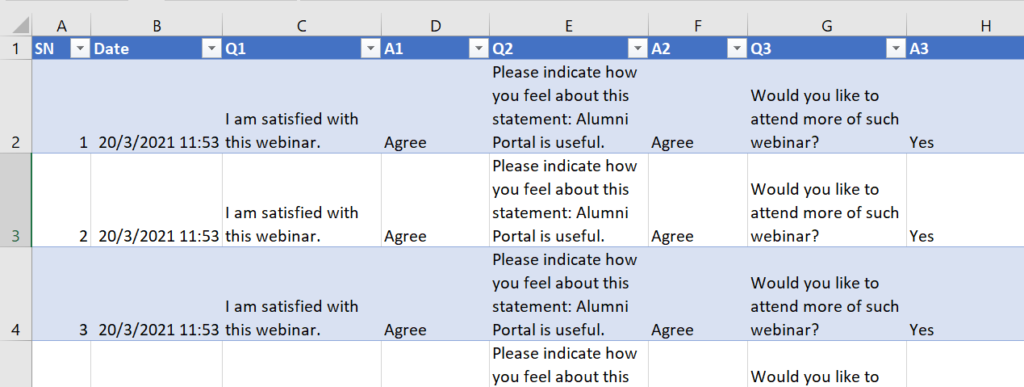
That is a very common mistake among Excel users.
The fault does not lie with Pivot Table. In fact, it is caused by the lack of knowledge from the user. To effectively analyze The problem with this survey result is that it is not able to analyze effectively with Pivot Table without re-arranging the data.
To create a Pivot Table that works, you have to make sure that the survey results are arranged this way (see below).
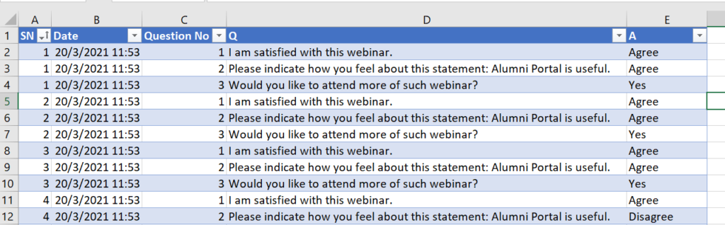
It cannot be done manually without doing lots of copy and paste. But with Power Query, it can be organized in less than a minute. Power Query is a new function in Excel and is available from Excel 2016 onwards. Here are the steps
- Go to the Data tab and click on “from table/range” icon. It would open the Power Query window.
- Select all the Questions and Answer Columns
- In the Power Query window, go to the Transform tab, and click on “Unpivot Columns”
- Split the Q and A column into 2 columns, one for the Q/A and another for the question no.
- Select the Q/A column
- Go to the transform tab and click on Pivot Column.
- In the setting that pop up, make sure you select Values as the value column and in the advanced setting, choose “Don’t Aggregate”.
- Go to the home tab and select “Close and Load to”.
- In the pop up window, select Pivot table.
- Organize the fields in the Pivot Table so that you can do a count straight away. Your report is completed and it should take you about 1 minute.
Watch this video below for the detailed steps: