HLOOKUP formula

Hlookup refers to Horizontal lookup. Its purpose is to look up a value or text horizontally across a row. When the value is found, it will return a value in another row that corresponds to the column of that value. Assuming that you have a table which presents the ages in the top row (header row) and the left column presents the height. In the table are the weight range that corresponds to the age and the height as shown below:

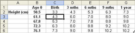
Using the formula, you can lookup the age (6 mths) across row 1. We will find 6 mths in column E. The formula can return any value below column E, depending on the value given in the formula. Here is how you should input the formula:

1. Select a blank cell.

2. Enter the formula (without the square brackets) "=Hlookup("6 mths",$B1:$G6,4,false)".

3. The formula will look for the value "6 mths" in the 1st row $B1:$G1.

4. The horizontal position (Column E) will be captured.

5. The number 4 in the formula "....$B1:$G6,4,false)" indicates that the result to return, when the value "6 mths" is found, is in row 4 (the result returned is 7.8).

6. The false that follows is a switch, to indicate that the exactly value must be found. Without the false, it will return the closest value that is greater than the value to be found.

vlookup: another useful formula similar to hlookup