Listing non-blank cells (non-array)

Listing non-blank cells within a range can be easily achieved using the auto-filter. For that, you can google for “Excel Auto-filter” and learn more about it from the top 5 lisitng. In here, we are going to do a little more advanced stuff: listing the non-blank cells in another location, either in a range within the worksheet or in another worksheet.

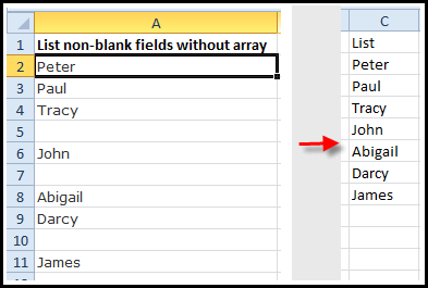
As shown in the picture below, there are some blank cells in between the range A2:A11.

And we want to use formulas to make it show a list without blanks in between (like the one on the right).

If you are just interested to copy and paste the formula into your worksheet without wanting to know how it is created, you can use this formula by change the ranges $A$2:$A$11 to your own range:

=IF(ROW(A1)>COUNTIF($A$2:$A$11,”>”””),””,INDEX($A$1:$A$11,SMALL(INDEX(($A$2:$A$11<>””)*ROW($A$2:$A$11),0),COUNTBLANK($A$2:$A$11)+ROW(A1))))

But if you wish to know how it works, continue reading.

First of all, let’s take a look at the formula. If I have the formula =ROW(A2) entered in a cell, it will return me the row number of A2, which is “2”. But if you list a range of cells from A2:A11, click inside the formula bar & press F9 to calculate =ROW($A$2:$A$11),it will list down all the numbers from 2 to 11.

But our objective is not to list down all the row numbers. We are only interested to show those rows that are not blanks, i.e. row 2, 3, 4, 6, 8, 9 & 11. To do that, we have to convert the rows which contain blank to show “0” instead. To do that, we can do a simple logical test to find out if the cells are blanks. (Logical test returns only 2 results, TRUE or FALSE.

=$A$2:$A$11<>””

Again, if you click inside the formula bar & press F9 to calculate, you will see that it creates a list of TRUEs & FALSEs. TRUE means the cell is not a blank, & FALSE means it is a blank:

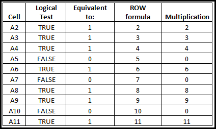
If you compare the positions of the TRUE and FALSE against the results generated by =ROW($A$2:$A$11), you will notice that the FALSE appeared in the same position as row number 5, 7 and 10 which are blank in column A.

In Excel, TRUE is actually equivalent to the value “1” and FALSE is “0”. So if we were to multiply this logical test =$A$2:$A$11<>”” with the ROW formula =ROW($A$2:$A$11), we will get “0” for those row numbers 5, 7 and 10 which contains blanks.

=($A$2:$A$11<>””)*ROW($A$2:$A$11)

This is what actually happened. A2 for eg, is not a blank. The logical test will turn “TRUE”, and “TRUE” is equivalent to the value “1”. The ROW of A2 is of course “2”, so the multiplication will be “1*2”, and returning “2”. This continues until a cell which has blanks (i.e. A5). The logical test turn “FALSE”, hence the value is “0”. Whatever the row number is, “0” multiplies by any number will return a “0”.

If we were to rank the numbers after the multiplication, “0” would be the smallest. 2nd and 3rd smallest numbers are still the other 2 zeroes. So the first value (Row number 2) on my list should be the 4th smallest row number, and the second value on my list should be the 5th, and so on. To get the number “4”, I can use COUNTBLANK to count how many “0”s I have.

=COUNTBLANK($A$2:$A$11)

That will give me a result of “3”. My list will be incremental by 1 as it goes down (i.e. 4th smallest, 5th smallest, etc). Thus, I can use the ROW formula again to add incremental value of 1

=COUNTBLANK($A$2:$A$11)+ROW(A1)

To find the nth smallest number (in a set of numbers), we can use the SMALL formula. The array would be our logical test and the ROW number combined together ($A$2:$A$11<>””)*ROW($A$2:$A$11). The “k” would be our COUNTBLANK and ROW formula:

=SMALL(($A$2:$A$11<>””)*ROW($A$2:$A$11),COUNTBLANK($A$2:$A$11)+ROW(A1))

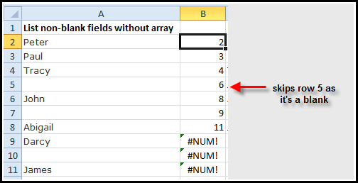
This formula above is good enough for an array formula. If you press CTRL + SHIFT + ENTER inside the formula bar, “2” should appear. And that’s actually referring to Row 2. Copy the formula down and you should see Cell B5 skip from row 4 to 6. This is because the next number ranked (in ascending orders) after 4 is 6. Row number 5 (meant for row 5 is converted to zero in our formula ($A$2:$A$11<>””)*ROW($A$2:$A$11)) is not in the list of numbers. Row 7 and 10 is also excluded when copied down.

As you can see, we have been pressing F9 inside the formula bar to get the results we want. These are array values, mostly to combine with array formulas (requires the curly bracket – created by using CTRL + SHIFT + ENTER to enter the formula). But we actually can park this array of values in the INDEX formula in order not to make this an array formula, i.e. don’t have to hit CTRL + SHIFT + ENTER to capture the formula with curly brackets. The arguments of the INDEX formula go like this:

We normally fill in the “row_num” or “column_num” as a number equals or more than 1. This will return us a single value from the “array” chosen. But if we were to put in “0” in either of them, it will give us all the values of the “array”. Hope you recall this formula?

=($A$2:$A$11<>””)*ROW($A$2:$A$11)

We can then put this formula inside the INDEX formula and put a “0” in the “row_num” argument:

=INDEX(($A$2:$A$11<>””)*ROW($A$2:$A$11),0)

And applying this back in the SMALL formula, you don’t have to press CTRL + SHIFT + ENTER anymore:

=SMALL(INDEX(($A$2:$A$11<>””)*ROW($A$2:$A$11),0),

COUNTBLANK($A$2:$A$11)+ROW(A1))

=SMALL(INDEX(($A$2:$A$11<>””)*ROW($A$2:$A$11),0),COUNTBLANK($A$2:$A$11)+ROW(A1))

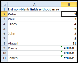
So column B should be showing the text in row 2 instead of the just the number 2. Also, the “#NUM!” error should be removed. It is appearing because in row 9, it is looking for the 11th smallest, but we only have 10 numbers from 2 to 11. Let’s do the text first. Since we have the row number, all we need is the INDEX formula for us to return the row of the array we state. (ALTernatively, you can also apply the OFFSET formula.) The ones in red are added to our existing formula (note the additional bracket at the end):

=INDEX($A$1:$A$11,SMALL(INDEX(($A$2:$A$11<>””)*ROW($A$2:$A$11),0),COUNTBLANK($A$2:$A$11)+ROW(A1)))

This is just to say from A1:A11, pick out the 2nd row. Copy down and you’ll have:

Now, to handle the errors, we have to find out how many cells are non-blank. COUNTA comes into mind, but this formula will fail if column A contains formulas that return blank cells. So we use this instead:

=COUNTIF($A$2:$A$11,”>”””)

This will return “7” as we have 7 non-blank cells. Our 8th value is the one with error, so we can say that if the nth value is greater than the number of non-blank cells, return blank. Otherwise, do the formula. To get the nth number, we can use ROW again. So:

=ROW(A1)>COUNTIF($A$2:$A$11,”>”””)

This is a logical test that will return TRUE or FALSE. Since ROW(A1) will return “1” and it is greater than 7, it will return FALSE. (Without the ROW(A1) formula, we will have to manual enter 1, 2, 3 into this part of the formula). Our IF statement will put a blank in the TRUE statement and the long formula we created, in the FALSE statement. This formula will only return “TRUE” when it is at ROW(A8) where “8” will be greater than 7. Using IF:

=IF(ROW(A1)>COUNTIF($A$2:$A$11,”>”””),””,

The formula after the comma is of course the long formula we created. Note the additional bracket at the end of the long formula.

=IF(ROW(A1)>COUNTIF($A$2:$A$11,”>”””),””,INDEX($A$1:$A$11,SMALL(INDEX(($A$2:$A$11<>””)*ROW($A$2:$A$11),0), COUNTBLANK($A$2:$A$11)+ROW(A1))))

That ends it!

Listing non-blank cells (non-array)

Popular Courses

Useful Links

Search the website