Answer to Questions submitted to Ask Jason Khoo
Question:
I have a workbook that contains 2 sheets. I have a column of records that I need Excel to consolidate to only unique records to the 2nd sheets. Then I am using the sumif command to total those. for example:
The first sheet has records in column B and C:
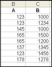
On the second sheet I only want to see
[supsystic-tables id=11]
I hope I made sense. I know about the Advanced filter for unique records, but I don’t want to have to re-run the filter everytime I update Sheet1. I would like it to run just like anyother formula.
Answer:
First you have identify the first instance of the number. When it appears, it should be given a number 1 unit larger than the last. The trunc formula will make sure that the decimals are not included in addition. If the number is a repeat, then add only 0.01 to the number. To make sure that this is possible, you need to make sure that you start counting from the beginning all the time and increase the range as it goes down. See diagram below:
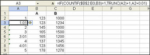
In the next sheet, start a series with an incremental of one. Then use vlookup to identify the value in the first sheet. Vlookup formula will return the value in the first sheet. Then do a sumif formula to find the total value related to the number found in the first sheet.
You can see the whole solution in this answer Hunter file
Question:
I am trying to build a report using sumif formula that will only pick up the “visible cells” when I filter the database. I am thinking of a combination sumif and subtotal formula to, in effect, change the target report everytime I filter the database. Any ideas?
Answer:
You need to use the subtotal formula and autofilter to accomplish the job. The subtotal will only sum/count those items that are visible
Question:
How to use the output of a cell close to the nearest two decimal in the equation of another (the figure has more than two decimals)?
Answer:
You can put the cell reference within the ROUND forumla to make use of the output rounded to two decimal places. For example, if the output (90.315) is presented in A1, and you want to double this value (90.32 – rounded to the nearest two decimal places) in cell A2, enter the formula in A2 as follows without the quotes “=A2*round(A1,2)” The 2 in round(A1,2) indicates the number of decimals to return in the formula. If you want to round it to the nearest tens, change the number 2 to -1. You can also use roundup and rounddown formulas instead of round.
Question:
I have downloaded a report from SAP to Excel. I tried to use HLOOKUP and VLOOKUP on the worksheet but they cannot work. The cell just displayed the formula in the cell. I have to save the file with prt extension before the 2 formulas worked.
Answer:
When you download the report from SAP, it could have converted all the cells in the worksheet to Text format. That why the formula appears in the cell. All you have to do is to select the entire worksheet and change the cell format to general before you apply your formulas.
Question:
I have inherited a spreadsheet whuch contains the following formula (and many more like it).
{=COUNT(IF((‘Build list’!$G$429=$B232)*(‘Build list’!L$429<>””)*(‘Build list’!$B$429<>””), (‘Build list’!$A$429)))}
My first question is what is the significance of {} around the function.
The second question is what does * do. It seems to act like ‘and’.
Regarding the { }, when I click on the function in the task bar they dissapear. If I press enter at this point the function stops working. If I press fx to test the function and then OK or clear the {} symbols remain. The values in columns G, L and B in the worksheet ‘Build List’ are correct. Column A has no values.
Answer:
1. The curly bracket {} indicate that the formula is an array formula. An array formula is used to perform calculation from 2 or more sets of value all at one go.
2. Asterisk (*) has two uses. One of the uses is to denote multiplcation. In your example, it is multipying (‘Build list’!$G$429=$B232) with (‘Build list’!L$429<>””). The second use is as a wildcard in text format. In the following sumif formula, it is to sum up all values in the range that start with the word Total. The wild card means it accepts any value after the word “Total” —
=SUMIF($B$2:$B$10,”Total*”, $C$2:$C$10).
See file attached.
The formula you inherit seems incorrect. Array formula usually involved a range like ‘Build list’!$G$2:$G$429 and not a single cell ‘Build list’!$G$429.
Copyright © advanced-excel.com 2007 – 2019. All Rights Reserved. Privacy Policy
Microsoft® and Microsoft Excel® are registered trademarks of Microsoft Corporation.
advanced-excel.com is in no way associated with Microsoft